 .
.
 .
. ,
,

 ,
or
,
or 
 and then you may
select parts and drag
them where you want them.
and then you may
select parts and drag
them where you want them.  ,
or
,
or 
 ,
or
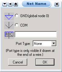
select "Edit/Label Net" from the menu.
,
or
select "Edit/Label Net" from the menu.
 on the tool bar (or any other way you normally save files).
  as usual.
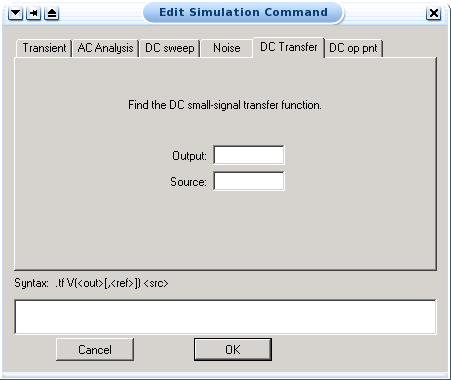
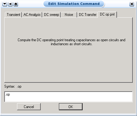
 or
use the "Simulate/Edit Simulation Menu" command.
or
use the "Simulate/Edit Simulation Menu" command.
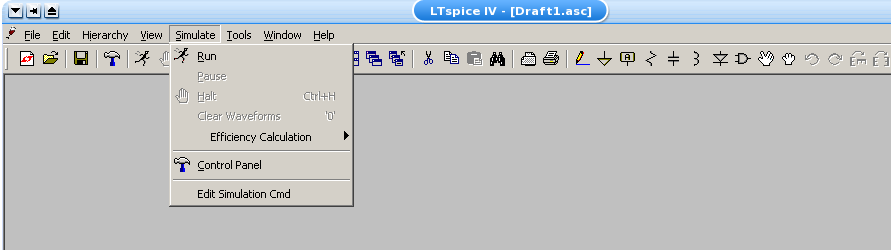 or
use the "Simulate/Run" command.
or
use the "Simulate/Run" command.

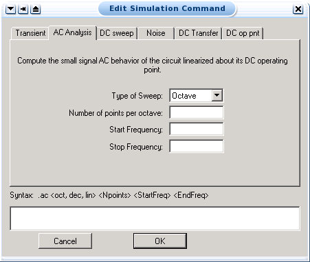
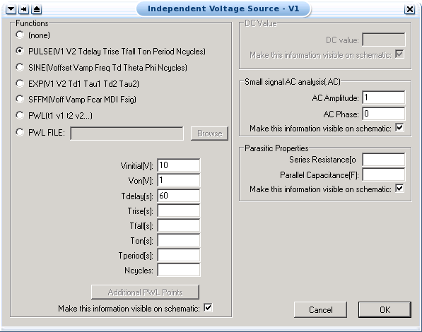
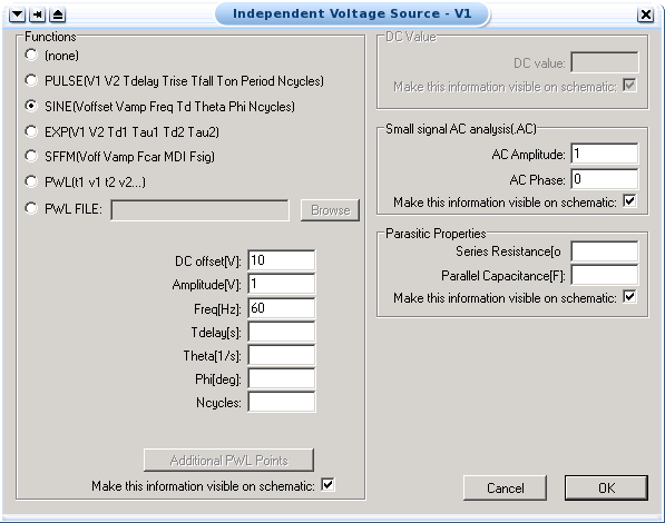
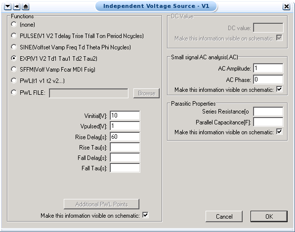
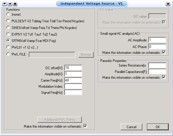
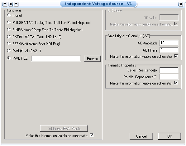
A voltage source can be configured in many possible ways. Right clicking on one will bring up the "Independent Voltag Source" window. The options which show up in the window will change as the function selected changes.
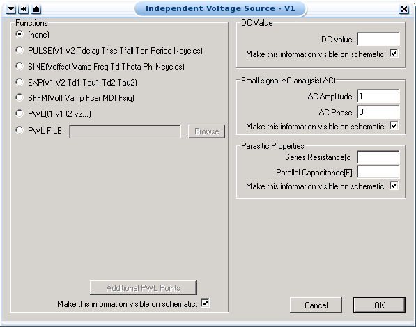
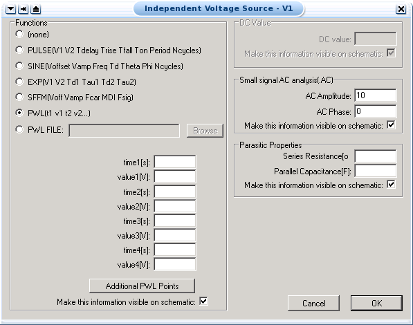
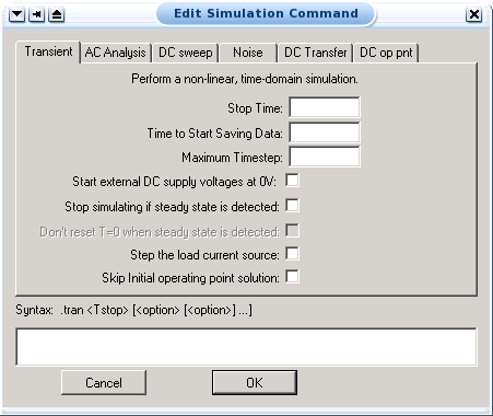
and fill it in with the Time Step that you want your 'clock' to have. This Time Step value is the your 'clock' pulse. There are various ways you can fill out the command prompts, one way is to do it as shown in the picture, however here are some simple commands that will allow you to do a range of simulations:
- REPEAT FOREVER, to simulate a real clock
- REPEAT <n> TIMES
- END REPEAT
- <<time>> INCR <<value>>
- <<time>> DECR <<value>>
- for <<value>> you can use, 0,1,R(rising), F(falling), X(unknown), or Z(high impedance)


Wilfrid Laurier University
© 2019 Wilfrid Laurier University
