Pages created and updated by Terry Sturtevant Date Posted: March 28, 2024

LTspice Tutorial

Introduction

While LTspice is a Windows program, it runs on Linux under Wine as well. (LTspice is also called SwitcherCAD by its manufacturer, since they use it primarily for the design of switch mode power supplies (SMPS).)
Note: Some of this was written using SwitcherCad III, and some was written using LTspice IV. The instructions should be the same.

On my YouTube channnel, I have a series of videos about LTspice.

Using LTspice

Opening LTspice
Drawing the circuit
Simulation
Simulation Commands
Types of Sources
1. Voltage Sources
  1. DC
  2. PULSE
  3. SINE
  4. EXP
  5. SFFM
  6. PWL
  7. PWL File
2. Current Sources
References and Links

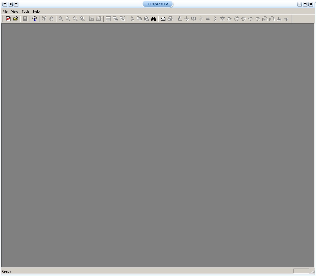
Opening LTspice:
- Find LTspice on the C-Drive. Open LTspice IV (or SWCad III). The opening screen will look like this:
  .
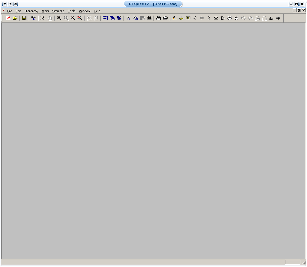
- Begin a new circuit
  - from the file menu, or
  - click on the "New Schematic" icon.
  Now you will see this:
  .
Drawing the circuit:
1. Adding a GND: This is very important. You cannot do any simulation on the circuit if you don't have a ground. To place a ground, you can
  - press the 'g' key, or
  - use the ground icon, , or
  - get it from the 'Edit' menu.
  If you aren't sure where to put it, place it near the bottom of the drawing.
2. Getting the other Parts:
  - The next thing that you have to do is get some or all of the parts you need.
  - This can be done by
    - clicking on the icon for a specific component;
      
      (This is good for common components such as resistors, capacitors, etc.)
    - clicking on the 'component' button; , or
    - pressing "F2"; or
    - going to "Edit" and selecting "Component..."
  - Once this box is open, select a part that you want in your circuit. This can be done by typing in the name or scrolling down the list until you find it.
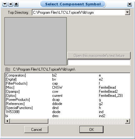
  - Some common parts are:
    - res - resistor
    - cap - capacitor
    - ind - inductor
    - diode - diode
    - voltage - any kind of power supply or battery
    Anything in [ ] is a library, which contains many parts.
  - To rotate parts so that they will fit in your circuit nicely, press "Ctrl+R" before placing the part. If you want to reflect (or 'Mirror') the part, press "Ctrl+E".
  - Upon selecting your parts, click where you want them placed (somewhere on the grey page with the dots). Don't worry about putting it in exactly the right place, it can always be moved later.
    Each type of part can be placed multiple times in succession, and they will be automatically numbered. when you want to stop placing a particular type of part, right-click or press 'Esc'.
3. Placing the Parts:
  - You should have most of the parts that you need at this point.
  - Now, all you do is put them in the places that make the most sense (usually a rectangle works well for simple circuits). To move parts, click on the 'move' icon, and then you may select parts and drag them where you want them.
    (When you have a part selected for a move, you can rotate or reflect it as well.)
  - If you have any parts left over, just select them and press "Delete".
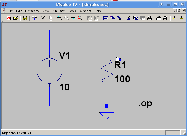
4. Connecting the Circuit:
  - Now that your parts are arranged well, you'll have to attach them with wires.
  - Go up to the tool bar and
    - select the "Draw Wire" button , or
    - "F3" or
    - go to "Edit" and select "Draw Wire".
  - With the pencil looking pointer, click on one end of a part, when you move your mouse around, you should see crossed lines appear. Attach the other end of your wire to the next part in the circuit.
  - Repeat this until your circuit is completely wired.
  - If you want to make a node (to make a wire go more then one place), click somewhere on the wire and then click to the part (or the other wire). Or you can go from the part to the wire. You should see a square block when 3 or more wires connect at a point.
  - Holding down CTRL while drawing lines allows you to make diagonal connections in the editor.
  - To get rid of the pencil, right click.
  - Mousing over a component allows you to edit its properties. Note the status bar in the lower left.
    
    The value of a component is one thing which can be edited.
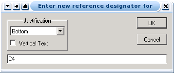
5. Changing the Name of the Part:
  - You probably don't want to keep the names C1, C2 etc., especially if you didn't put the parts in the most logical order. To change the name, right click on the present name (C1, or R1 or whatever your part is), then a box will pop up (Enter New Reference Designator), where you can type in the name you want the part to have.
  - Please note that if you double click on the part or its value, no box will appear.
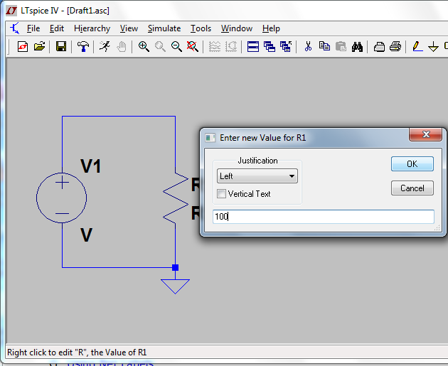
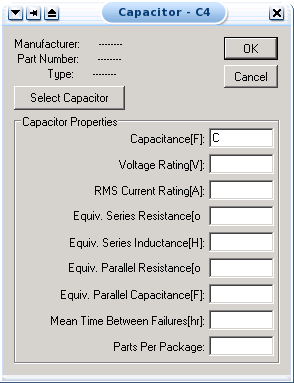
6. Changing the Value of the Part:
  - If you only want to change the value of the part (if you don't want all your resistors to be 1K ohms), you can right click on the part, (not the name), and a box title by the part name (such as "Resistor") will appear. The number of fields in the box will depend on the type of part it is. Type in the new value and press OK. Use u for micro as in uF = microFarad.
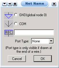
7. Using Net Labels:
  - These are important if you want to user your own identifiers for points in the network where you want to determine voltages rather than having to work with the node numbers that LTspice assigns.
  - To add net labels,
    - press "F4", or
    - click on the "Label Net" icon , or
    - select "Edit/Label Net" from the menu.
    When you do this, a window will pop up where you assign the label you want to use for the net.
8. Adding your own SPICE Models or Subcircuits
  
  How to add a model to LTspice (SwitcherCad)
  This assumes you want to add a new model for a new device similar to one in the existing library. Here are three different methods.
  
  Method 1: Modify Libraries
  This method makes sense if you are working on your own computer, where you can update your own libraries and use them again.
  1. Look under C:\Program Files\LTC\LTspiceIV
    (or C:\Program Files\LTC\SwCADIII )
  2. Go to the directory lib\cmp
  3. Look at the list of standard devices to figure out which kind you want, such as:
    - standard.bjt
    - standard.dio
    - standard.jft
    - ...etc...
    Each line in each of these files has a model for one device.
  4. Add a line with the .model line for your device to the end of the appropriate file using a text editor.
    Note you may have to adapt the model line to match the pattern in the file. It should be pretty easy to figure out.
  Now when you open LTSpice, you should be able to pick the device you've added as though it was one of the existing models.
  
  Method 2: Using an external library file
  This will work well if you are using a computer where you can't edit the built-in library files, or where edits will not be saved, but where you may have several models in one file which you would like to be able to use in the future.
  1. Save the file which contains the model you want to use in a directory where you have write access. (For example, I use c:\windows\temp.)
  2. Insert a SPICE directive from the edit menu,
    
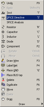
    by using the icon, or by typing 'S'.
    In the text box, type
    .lib path to your library file
    so, for example
    .lib c:\windows\temp\myfile.sp3
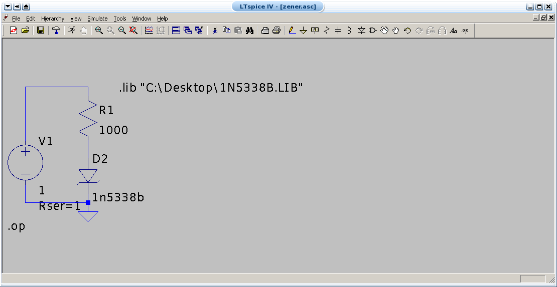
  3. Change the name of the component in your schematic to match the exact name of the model in the library file.
  Now when you simulate, your new device model should be used.
  Note: you can use the .include directive instead of the .lib directive if you wish.
  
  Method 3: Inserting the model directly into the drawing
  This will work well if you are using a computer where you can't edit the built-in library files, or where edits will not be saved, and that there is only a single model you want to use.
  1. Open file which contains the model you want to use, and copy the model into the clipboard.
  2. Insert a SPICE directive from the edit menu, by using the icon, or by typing 'S'.
    In the text box, paste the model from the clipboard.
  3. Change the name of the component in your schematic to match the exact name of the model in the model line.
  Now when you simulate, your new device model should be used.
  Note: Because you now have the model saved as part of your schematic, this is completely portable between computers.
  
  How to add a subcircuit model to LTspice (SwitcherCad)
  Sometimes you need to add something which is more complicated than simply a model.
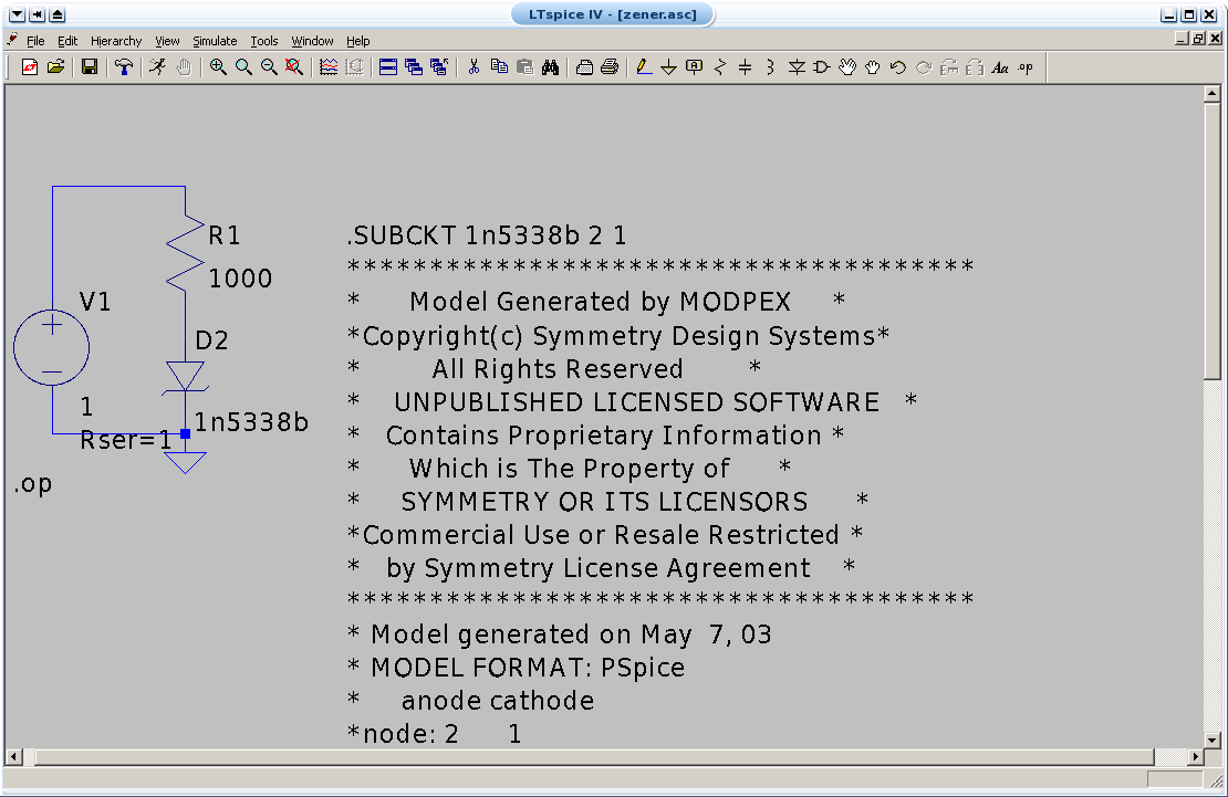
  In this case you can add add a subcircuit model for a device. You'll save a bit of time if the new device at least looks similar to one in the existing library. Otherwise you may have to draw a new symbol. (Suppose the file that contains the model you want to use is called 1N5338B.LIB and the model you want to use is a subcircuit called 1N5338B.)
  Method 1: Modify Libraries
  This method makes sense if you are working on your own computer, where you can update your own libraries and use them again.
  1. Look under C:\Program Files\LTC\LTspiceIV
    (or C:\Program Files\LTC\SwCADIII )
  2. Put the file 1N5338B.LIB in the subdirectory lib\sub .
  3. Go to the directory lib\sym
  4. Find a component similar to what you want. That way you won't have to draw the symbol from scratch. For instance, if I were adding a new zener diode, I see there's a component zener.asy.
  5. Copy zener.asy to 1N5338B.asy. (1N5338B will be the name of the new zener diode model I want to use.)
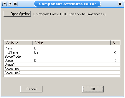
  6. Open 1N5338B.asy in a text editor, and make the following changes:
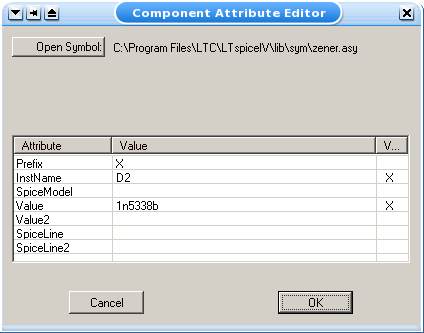
    - change SYMATTR Prefix D to SYMATTR Prefix X
      (This says that the model we're using is a .subckt.)
    - change SYMATTR Value D to SYMATTR Value 1N5338B
      (This says that the name that will show up on the schematic is 1N5338B.)
    - add a line SYMATTR ModelFile 1N5338B.LIB
      (This says that the name of the file containing the subcircuit we're using is 1N5338B.LIB.)
    - add a line SYMATTR SpiceModel 1N5338B
      (This says that the name of the subcircuit we're using is 1N5338B. You can see this by looking at the first line of the file:
      .SUBCKT 1n5338b 2 1
      This tells the name of the subcircuit and that it has two pins.)
  Now when you open LTSpice, you should be able to find the component you have added, and use it like any of the ones that are built-in .
  Method 2 and Method 3: Setup
  This same procedure applies to both methods. These methods will be useful where you can't edit the library files. This might happen if you are working on computers in public labs, for instance.
  1. Hold down CTRL-M while right-clicking on the component to bring up the dialog.
  2. Change the prefix of the device to "X" to indicate you are using a subcircuit, and edit the value of the device to match the subcircuit name exactly.
  After these steps, go on to either Method 2 or Method 3.
  Method 2: Using an external library file
  This will work well if you are using a computer where you can't edit the built-in library files, or where edits will not be saved, but where you may have several models in one file which you would like to be able to use in the future.
  1. Save the file which contains the subcircuit you want to use in a directory where you have write access. (For example, I use c:\windows\temp.)
  2. Insert a SPICE directive from the edit menu,
    
    by using the icon, or by typing 'S'.
    In the text box, type
    .lib path to your library file
    so, for example
    .lib c:\windows\temp\myfile.sp3
  Method 3: Inserting the model directly into the drawing
  This will work well if you are using a computer where you can't edit the built-in library files, or where edits will not be saved, and that there is only a single model you want to use.
  1. Open file which contains the subcircuit you want to use, and copy the subcircuit into the clipboard.
  2. Insert a SPICE directive from the edit menu, by using the icon, or by typing 'S'.
    In the text box, paste the subcircuit from the clipboard.
    
    The subbcircuit itself may include model definitions, so you may have to include several lines when you copy. If the library file is only for that one device, then you'll want to copy and paste the entire file contents.
9. Saving:
  - To save the circuit, use the save button on the tool bar or any other method you would normally use to save files.
10. Printing:
  - To print, you may use the menu or the print icon as usual.
Simulation:
1. Before you do the simulation:
  - You have to have your circuit properly drawn and saved.
  - There must not be any floating parts on your page (i.e. unattached devices).
  - You should make sure that all parts have the values that you want.
  - There are no extra wires.
  - It is essential that you have a ground in your circuit.
2. Choosing a simulation:
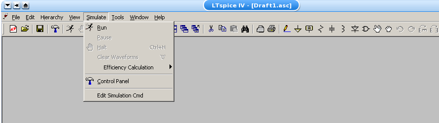
  - Click on the Simulate button on the tool bar or use the "Simulate/Edit Simulation Cmd" command.
  - Enable whatever type(s) of analysis you want using the Edit Simulation Command window. The last one you choose is the one which will be done when you simulate.
  - Click on the Simulate button on the tool bar or use the "Simulate/Run" command.
  - It will check to make sure you don't have any errors. If you do have errors, correct them.
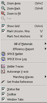
3. Graphing:
  - Go to the "View" menu:
4. Adding/Deleting Traces:
  - Use "Visible Traces" or on the toolbar to select all the traces you want.
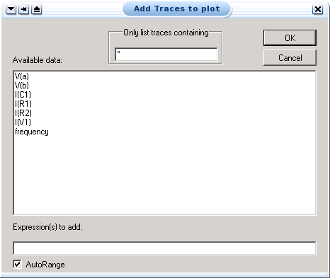
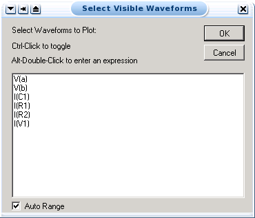
  - The add traces window allows you to choose various signals from the circuit, or to create mathematical expressions involving them.
  - To delete a trace, select its title on the graph and press "Delete".
5. Doing Math:
  - In Visible Traces, there are functions that can be performed, these will add/subtract (or whatever you chose) the lines together.
  - Select the signal(s) that you wish to have displayed.
  - There are many functions here that may or may not be useful. If you want to know how to use them, you can use LTspice's Help Menu.
6. Labeling:
  - Click on Text Label
    on top tool bar.
  - Type in what you want to write.
  - Click OK
  - You can move this around by single clicking and dragging.
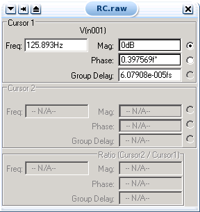
7. Finding Points: (aka Using Cursors)
  - Click on the name of the trace you want to look at and then a cursor window will appear, showing information about the point currently selected.
    .
    Note that if you right click on the trace name, you can choose to show two cursors. This then allows automatic math to be done, such as to give the difference between them in both dimensions.
  - You can use the cursor keys to move back and forth through the data points.
8. Changing the horizontal axis variable
  - Move the mouse over the horizontal axis until you see the cursor change.
    .
    At the bottom of the screen, you should see the following message.
    .
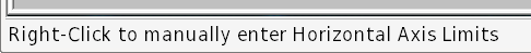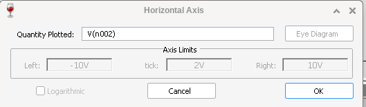
  - Right-clicking will bring up a dialog.
    .
    
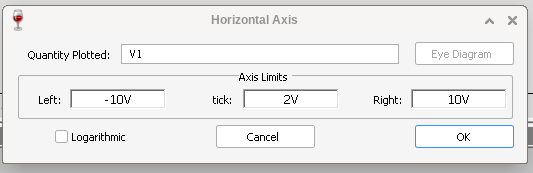    You can change the "Quantity Plotted" to any variable, such as a node voltage or device current.
    .
9. Saving:
  - To save your probe you need to go into the tools menu and click display, this will open up a menu which will allow you to name the probe file and choose where to save it. You can also open previously saved plots from here as well.
10. Printing:
  - Select Print in Edit or on the toolbar .
  - Print as usual.
Simulation Commands
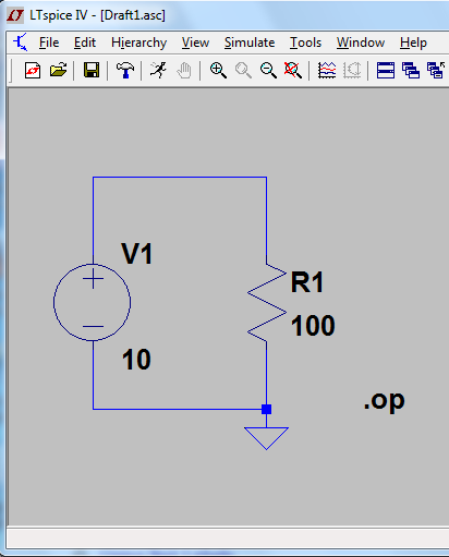
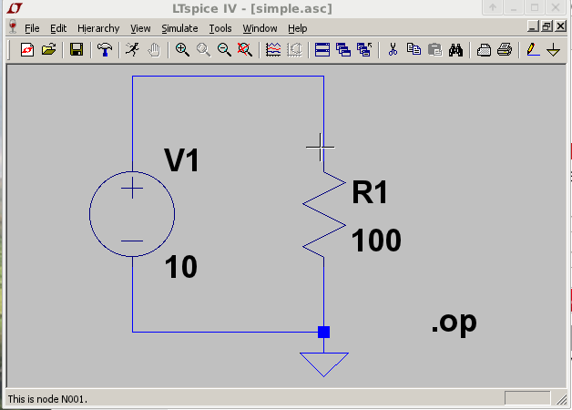
1. DC Operating Point
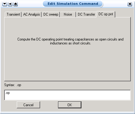
  - This is a simple, but incredibly useful analysis. It will not give you anything to plot, but it will indicate the DC voltages at all nodes and DC currents through all devices in the circuit.
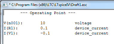
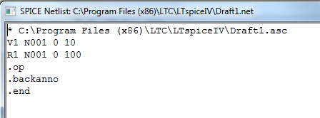
  - The output of the simulation is a very simple text file.
    
    After a simulation has been performed, mousing over any wire in the circuit will show what node it belongs to in the status bar. (See the lower left corner of the screen.)
    
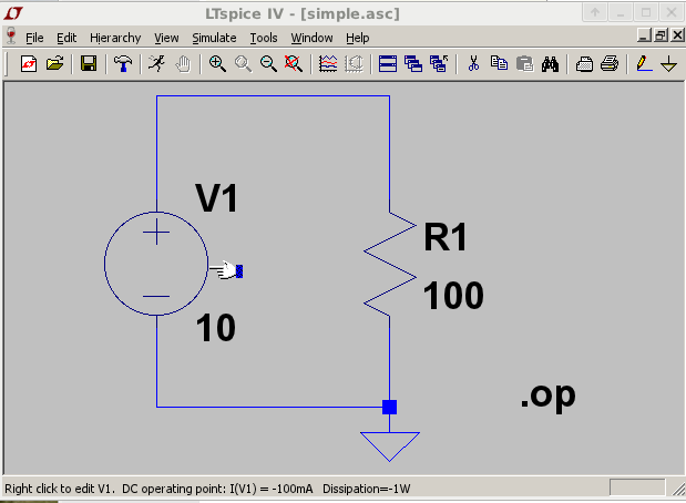
    After a simulation has been performed, mousing over a component shows parameters like current and power in the status bar.
    
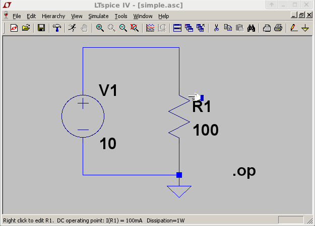
    Note the sign of the current and power from the source.
    
    You can view the netlist from the menu.
    
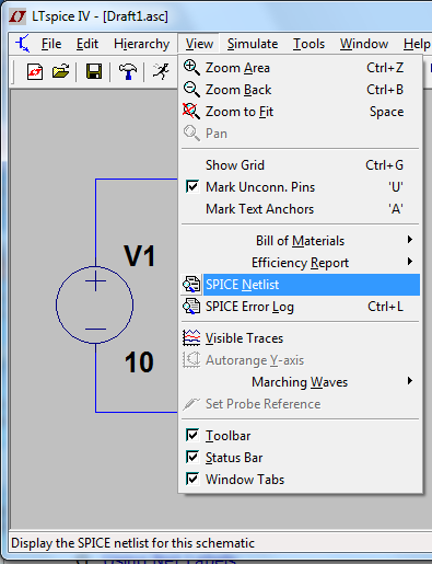
    The netlist allows you to see the node numbers for each device, among other things.
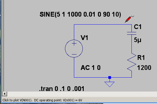
2. Transient
  
  When doing a transient analysis of a source, the sections highlighted below in the source configuration window are relevant.
  
  Here's the simulation command window:
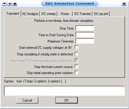
  - The transient analysis is probably the most important analysis you can run in LTspice, and it computes various values of your circuit over time. Two very important parameters in the transient analysis are:
    - Stop Time.
    - Time to Start Saving Data
    - Maximum Timestep
    - (various checkboxes....later)
  - The ratio of Stop Time: Maximum Timestep determines how many calculations LTspice must make to plot a wave form. LTspice always defaults the start time to zero seconds and going until it reaches the user defined final time. It is incredibly important that you think about what timestep you should use before running the simulation, if you make the timestep too small the probe screen will be cluttered with unnecessary points making it hard to read, and taking extreme amounts of time for LTspice to calculate. However, at the opposite side of that coin is the problem that if you set the timestep too high you might miss important phenomenon that are occurring over very short periods of time in the circuit. Therefore play with step time to see what works best for your circuit.
  - You can set a step ceiling which will limit the size of each interval, thus increasing calculation speed. Another handy feature is the Fourier analysis, which allows you to specify your fundamental frequency and the number of harmonics you wish to see on the plot. LTspice defaults to the 9th harmonic unless you specify otherwise, but this still will allow you to decompose a square wave to see it's components with sufficient detail.
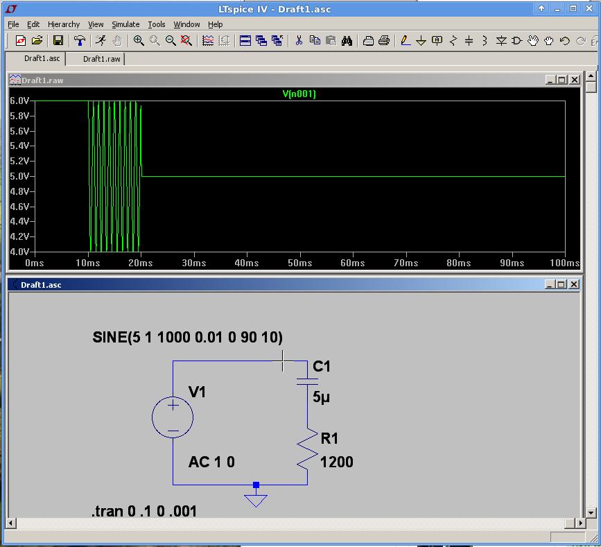
  - You can look at the signal at any node.
    
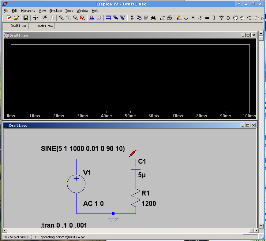
    Note the status bar shows more information.
    
    The output shows up like this..
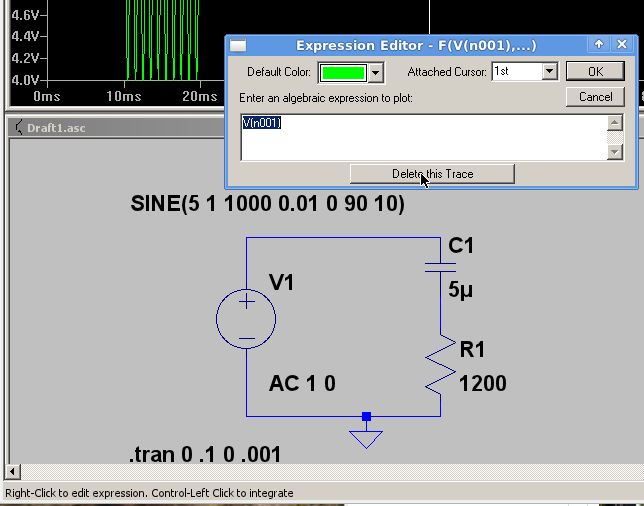
  - You can delete or modify any signal.
    
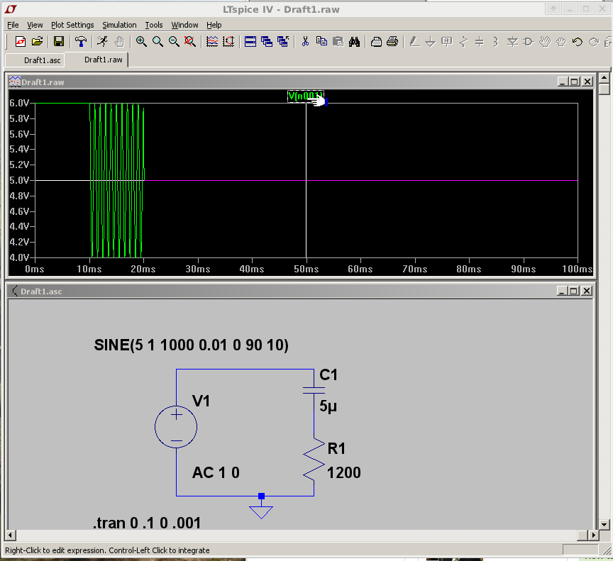
    The dialog allows various changes.
    
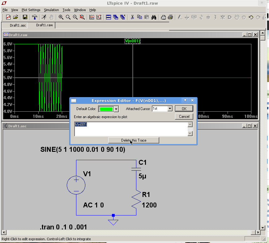
    Note the status bar shows more information.
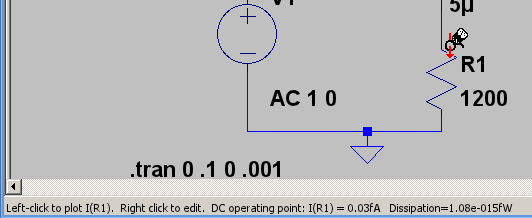
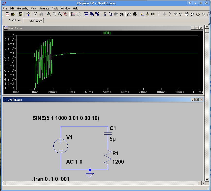
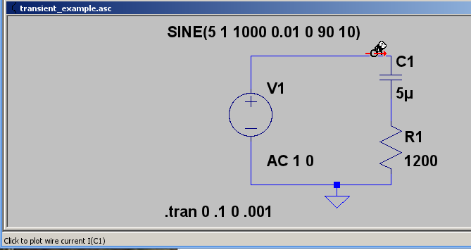
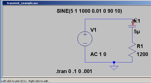
  - You can look at the current through any device.
    
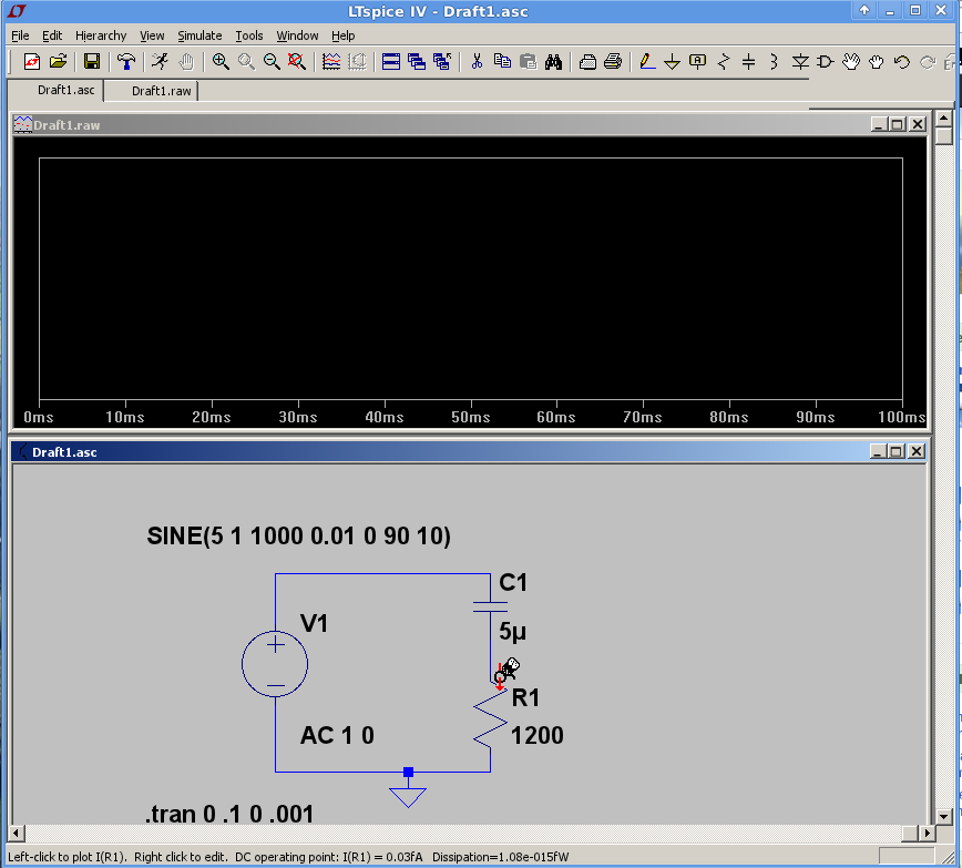
    Note the status bar shows more information.
    
    The output shows up like this..
  - You can also look at the current through any wire. Remember you get the voltage by mousing over any point in a node, (such as along a wire).
    
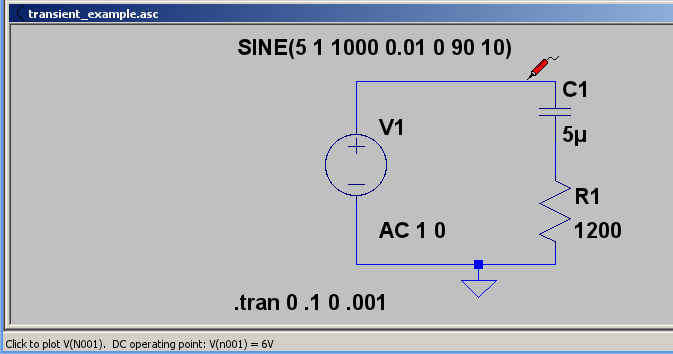
    Now, if while mousing over it you hold down the ALT key, you'll see the current pointer and the status bar indicates you can click to plot the wire current.
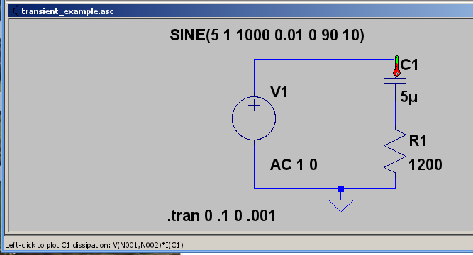
  - You can also look at the power dissipation in any device. Remember you get the current by mousing over any device.
    
    Now, if while mousing over it you hold down the ALT key, you'll see the power pointer, (a thermometer), and the status bar will show you can plot the device power dissipation.
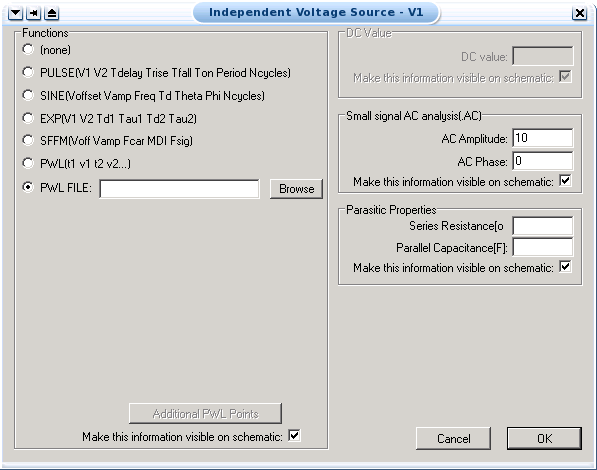
3. AC Analysis
  
  When doing an AC sweep of a source, the sections highlighted below in the source configuration window are relevant.
  Note: In an AC sweep, all AC sources are treated as sine waves.
  
  Here's the simulation command window:
  
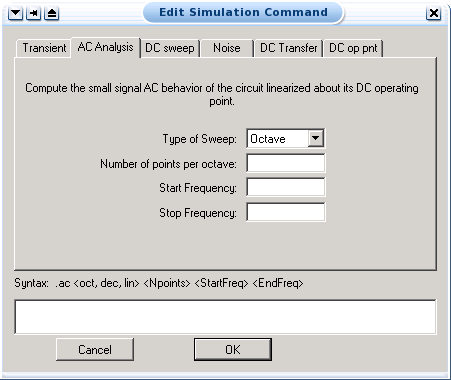
  The AC analysis allows you to plot magnitude and/or phase versus frequency for different inputs in your circuit.
  - Type of Sweep
    In the AC analysis menu you have the choice of three types of analysis:
    - Linear,
    - Octave and
    - Decade.
    These three choices describe the X-axis scaling which will be produced in probe. For example, if you choose decade then a sample of your X-axis might be 10Hz, 1kHz, 100kHz, 10MHz, etc.... Therefore if you want to see how your circuit reacts over a very large range of frequencies choose the decade option.
  - You now have to specify at how many points you want LTspice to calculate frequencies, and what the start and end frequency will be. That is, over what range of frequencies do you want to simulate your circuit.
    - Number of points
    - Start Frequency
    - Stop Frequency
4. DC Sweep
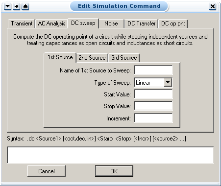
  - The DC sweep allows you to do various different sweeps of your circuit to see how it responds to various conditions.
  - For all the possible sweeps,
    - voltage,
    - current
    you need to specify a start value, an end value, and the number of points you wish to calculate.
  - For example you can sweep your circuit over a voltage range from 0 to 12 volts. The main two sweeps that will be most important to us at this stage are the voltage sweep and the current sweep. For these two, you need to indicate to LTspice what component you wish to sweep, for example V1 or V2.
  - Another excellent feature of the DC sweep in LTspice, is the ability to do a nested sweep.
  - A nested sweep allows you to run two simultaneous sweeps to see how changes in two different DC sources will affect your circuit.
  - Once you've filled in the main sweep menu, click on the nested sweep button and choose the second type of source to sweep and name it, also specifying the start and end values. (Note: In some versions of LTspice you need to click on enable nested sweep). Again you can choose Linear, Octave or Decade, but also you can indicate your own list of values, example: 1V 10V 20V. DO NOT separate the values with commas.
5. Noise
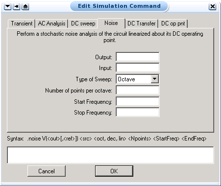
  - LTspice will simulate noise for you either on the output or the input of the circuit. These noise calculations are performed at each frequency step and can be plotted in probe.
  - The two types of noise are:
    - Output for noise on the outputs and
    - Input for noise on the input source.
    - Type of Sweep (same as for AC analysis)
    - Number of points... (same as for AC analysis)
    - Start Frequency (same as for AC analysis)
    - Stop Frequency (same as for AC analysis)
  - To use input noise you need to tell LTspice where you consider the 'input' in your circuit to be, for example, if your voltage source is labeled 'V1'.
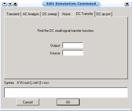
6. DC Transfer
7. Parametric
  - Parametric analysis allows you to run another type of analysis (DC operating point, transient, sweeps) while using a range of component values. The best way to demonstrate this is with an example, we will use a resistor, but any other standard part would work just as well (capacitor, inductor).
  - First, right click the value resistor that is to be varied. This will open a dialog box allowing you to set "Resistor Properties". Enter the name {R} (including the curly braces) in place of the component value.
    
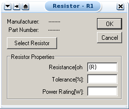
    This indicates to LTspice that the value of the resistor is a global parameter called R.
  - Now add a spice directive to the page, by pressing the 's' key, using the icon
    
    or the menu command
    
    Place the box anywhere on the schematic page.
  - Edit the directive.
    
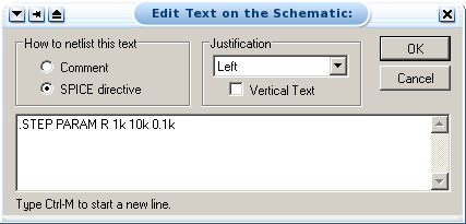
    Directives always start with a period.
    .STEP PARAM R 1k 10k 0.1k means to step the parameter R from 1kΩ to 10kΩ in steps of 0.1kΩ for every step of the outer simulation.
  - You'll need to have one simulation command, even if it's a DC operating point analysis.
    Choose an analysis as usual, and run the simulation.
  - If your did a non-graphical analysis, such as a DC operating point, then you'll get a graphical output which has the stepped parameter as the horizontal axis.
    If you did an analysis that is already graphical, such as transient, you'll get a graph with a series of lines, one for each value of the stepped parameter. In order to isolate one trace,
    
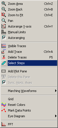
    use the command to "Select Steps" from the trace menu. This brings up a dialog
    
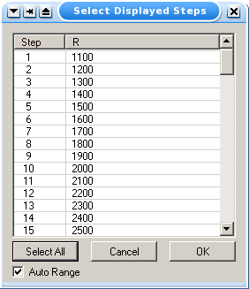
    which allows you to choose which one(s) you want to show.
8. Temperature
  - To do a temperature sweep, do a parametric analysis but instead of varying a component value, vary the temperature as follows:
    .STEP TEMP 0 100 1 means to step the temperature from 0°C to 100°C in steps of 1°C for every step of the outer simulation.
9. Other types of analysis There are other SPICE analyses possible. Eventually I might get them in here, including
  - fourier
Types of Sources
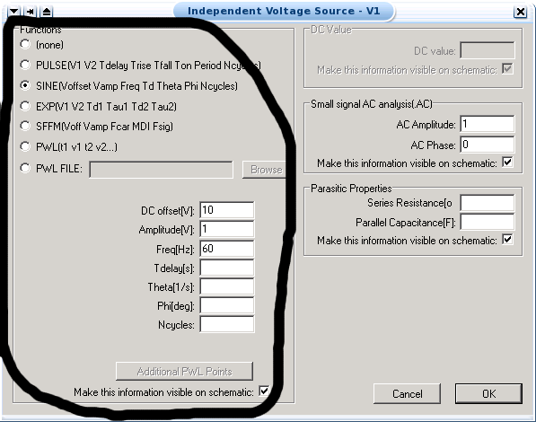
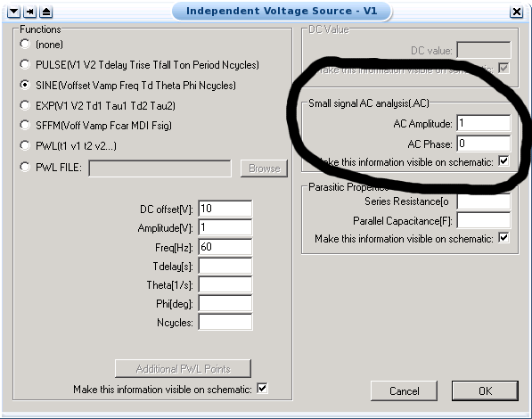
1. Voltage Sources A voltage source can be configured in many possible ways. Right clicking on one will bring up the "Independent Voltage Source" window. The options which show up in the window will change as the function selected changes.
  1. (none)
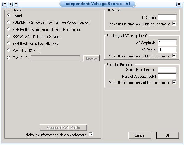
    - This is your basic direct current voltage source that simulates a simple battery and allows you to specify the DC voltage value.
  2. PULSE
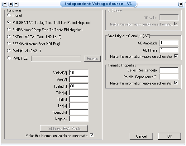
    - PULSE is often used for a transient simulation of a circuit where we want to make it act like a square wave source. It should never be used in a frequency response study because LTspice assumes it is in the time domain, and therefore your probe plot will give you inaccurate results.
      - V_initial is the value when the pulse is not "on." So for a square wave, the value when the wave is 'low'. This can be zero or negative as required. For a pulsed current source, the units would be "amps" instead of "volts."
      - V_on is the value when the pulse is fully turned 'on'. This can also be zero or negative. (Obviously, V₁ and V₂ should not be equal.) Again, the units would be "amps" if this were a current pulse.
      - T_delay is the time delay. The default units are seconds. The time delay may be zero, but not negative.
      - T_rise is the rise time of the pulse. LTspice allows this value to be zero, but zero rise time may cause convergence problems in some transient analysis simulations. The default units are seconds.
      - T_fall is the fall time in seconds of the pulse.
      - T_on is the pulse width. This is the time in seconds that the pulse is fully on.
      - T_period is the period and is the total time in seconds of the pulse.
      - N_cycles is the number of cycles of the pulse that should happen. Leave it as zero if you want ongoing pulses.
    - This is a very important source for us because we do a lot of work with the square wave on the wave generator to see how various components and circuits respond to it.
  3. SINE
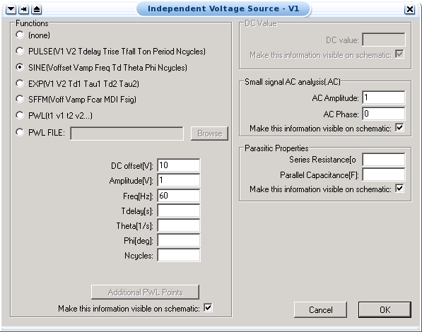
    - A few things to note about the alternating current source. First, there are two possible analyses which can be done and so there are two sets of parameters.
      For an ac analysis, the parameters are:
      - AC Amplitude which is the peak value of the voltage.
      - AC Phase which is the phase angle of the voltage
      For a transient analysis, the parameters are:
      - DC offset is the DC offset voltage. It should be set to zero if you need a pure sinusoid.
      - Amplitude is the undamped amplitude of the sinusoid; i.e., the peak value measured from zero no DC offset value.
      - Freq is the frequency in Hz of the sinusoid.
      - T_delay is the time delay in seconds. Set this to zero for the normal sinusoid.
      - Theta is the damping factor. (Not the phase angle!) Also set this to zero for the normal sinusoid.
        This is used to apply an exponential decay to the sinusoid; theta is the decay constant in 1/seconds.
      - PHI is the phase advance in degrees. Set this to 90 if you need a cosine wave form.
      - N_cycles is the number of cycles of the pulse that should happen. Leave it as zero if you want ongoing pulses.
      For this analysis, LTspice takes it to be a sine source, so if you want to simulate a cosine wave you need to add (or subtract) a 90° phase shift. Note that the phase angle if left unspecified will be set by default to 0°
  4. EXP
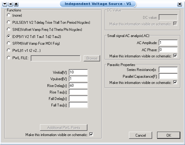
    - The EXP type of source is an exponential voltage, illustrated here:
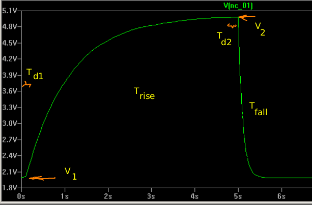
      - Vinitial the starting voltage, V₁
      - Vpulsed the maximum voltage, V₂
      - Rise Delay the time to wait at the starting voltage before changing, T_d1
      - Rise Tau the time constant for the change, Tau₁
      - Fall Delay the time to wait at the maximum voltage before changing, T_d2
      - Fall Tau the time constant for the change back to the starting voltage, Tau₂
  5. SFFM
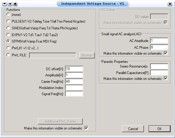
    - The SFFM (Single Frequency FM) type of source has these parameters:
      - DC offset the DC component of the sine wave
      - Amplitude the AC value of the sine wave
      - Carrier Freq is the carrier frequency.
      - Modulation Index is the modulation index.
      - Signal Freq is the signal frequency.
  6. PWL (Piece-Wise Linear)
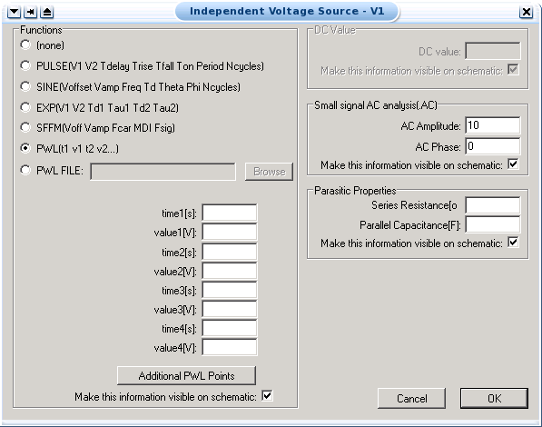
    - The PWL source is a Piece Wise Linear function that you can use to create a wave form consisting of straight line segments drawn by linear interpolation between points that you define. Since you can use as many points as you want, you can create a very complex wave form This source type can be a voltage source or a current source.
    - The syntax for this source type is flexible and has several optional parameters. The required parameters are two-dimensional points consisting of a time value and a voltage (or current) value. There can be many of these data pairs, but the time values must be in ascending order, and the intervals between time values need not be regular.
  7. PWL File
    - The PWL File source reads a file for Piece Wise Linear function parameters.
2. Current Sources
  - For each of the previous discussed voltage sources, there exists the exact same source except that it produces current. There is one thing that should be mentioned; current sources in LTspice get a little confusing. For those current sources whose circuit symbol has an arrow, you have to point the arrow in the direction of conventionally flowing current. This applies to all current sources, including AC and DC. Therefore placing the current source in the circuit backwards with seemingly incorrect polarities will give the correct results.
  - An interesting little feature under the markers menu is the ability to add markers to your circuit so you can see where the current and voltage have imaginary values in the circuit, and the phase of your source at any point in the circuit.
References and Links
1. Introduction to SwitcherCAD (another name for LTspice) [PDF; Petr Kropik]
  This has a good step-by-step guide, including information about files and SPICE directives.
2. LTSpice introductory manual (adding components) [PDF; Aalborg University, October 2005]
  This has useful information about how to add libraries and models.
3. SPICE overview (lots of detail) [University of Pennsylvania]
  Since this is about SPICE itself, rather than any particular version, such as PSpice or LTspice, the information is very widely applicable.
4. SWCADIII (Another LTspice tutorial) (very detailed) [PDF; Aalborg University]
  This starts off with a lot about Switch Mode Power Supplies, i.e. what Linear Technology designed it for, but gets into lots of other stuff as well. (It's 257 pages long, so there really is a lot of stuff there.
5. Intro to LTspice (lots of screen shots) [PDF; South Dakota School of Mines and Technology]
  Shorter than some of the others, but lots of screen shots
6. Other kinds of analysis (blog) [ Chris Cross]
  This includes an example of varying temperature for an analysis.
7. Diagonal symbols (for common components; resistor, capacitor, inductor, didode)
  I think that sometimes it would be nice to be able to draw things like bridge circuits in the way they're normally shown, rather than with all components either horizontal or vertical, so I created diagonal versions of the basic components.
  (Holding down CTRL while drawing lines allows you to make diagonal connections in the editor.)
8. McGraw-Hill tutorial that includes a PowerPoint presentation and lots of circuit files.
9. For the more obscure questions you might have go right to the source at Linear Technology©
  http://www.linear.com/designtools/software/#LTspice
10. There's a Yahoo! group which is quite active with discussions, examples etc.
  https://groups.yahoo.com/neo/groups/LTspice/info
11. Another site with useful tutorials
  http://www.zen22142.zen.co.uk/ltspice/ltindex.htm
  DC circuits introduction
  http://www.zen22142.zen.co.uk/ltspice/dccircuits.htm

**Most of the pictures and screen shots came from Linear Technology© LTspice version 4.08o

Not related to LTspice specifically, but there is a tutorial on using LaTeX to typeset technical documents at
http://denethor.wlu.ca/latex/

LTspice Tutorial

Introduction

Using LTspice

Opening LTspice

Drawing the circuit

Simulation

Simulation Commands

Types of Sources

References and Links

How to add a model to LTspice (SwitcherCad)

Method 1: Modify Libraries

Method 2: Using an external library file

Method 3: Inserting the model directly into the drawing

How to add a subcircuit model to LTspice (SwitcherCad)

Method 1: Modify Libraries

Method 2 and Method 3: Setup

Method 2: Using an external library file

Method 3: Inserting the model directly into the drawing

Resources